Plotting FLEXPART trajectories in 3D terrain map

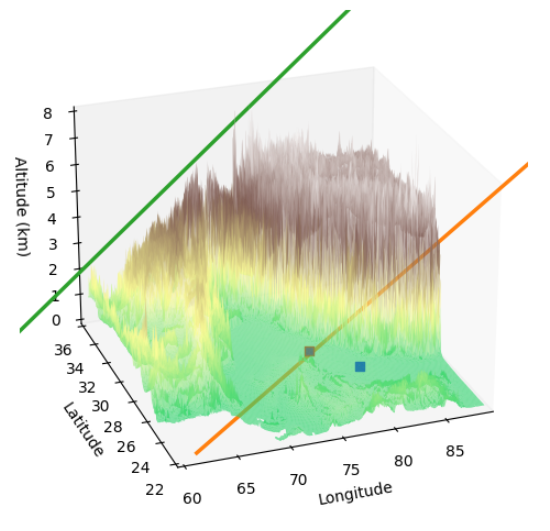
This blog post demonstrates how to plot FLEXPART model trajectories on a 3D terrain map, integrating topography and transport data for enhanced visualization. The workflow includes:

• Loading terrain data
• Plotting air mass trajectories in 3D
• Creating illustrative particle dispersion effects

1. Load and Visualize Terrain Data

import numpy as np
import matplotlib.pyplot as plt
from mpl_toolkits.mplot3d import Axes3D
import cartopy.crs as ccrs
import cartopy.feature as cfeature
from cartopy.io import shapereader
from netCDF4 import Dataset

# load the terrain file
etopo_file = "./../../../../../4.Punjab_fire/Analysis_notebook/ETOPO_2022_v1_60s_N90W180_bed.nc"  # Replace with your local ETOPO1 file
nc = Dataset(etopo_file)
# Extract data from ETOPO1
lon = nc.variables['lon'][:]
lat = nc.variables['lat'][:]
elevation = nc.variables['z'][:]

# Mask the ocean by setting all elevation <= 0 (sea level or below) to NaN
elevation_masked = np.where(elevation <= 0, np.nan, elevation)


# Extract the topo data to the area of interest
lon_min, lon_max = 60, 89
lat_min, lat_max = 22, 36
lon_indices = np.where((lon >= lon_min) & (lon <= lon_max))[0]
lat_indices = np.where((lat >= lat_min) & (lat <= lat_max))[0]

subset_lon = lon[lon_indices]
subset_lat = lat[lat_indices]
subset_elevation = elevation_masked[np.ix_(lat_indices, lon_indices)]

lon_grid, lat_grid = np.meshgrid(subset_lon,subset_lat)

# Normalize elevation data for better 3D visualization
elevation_normalized = np.clip(subset_elevation/ 1000, 0, subset_elevation.max()/1000.0)  # Convert to km


from matplotlib.colors import LinearSegmentedColormap
import shapefile
from shapely.geometry import Polygon
from shapely.geometry import mapping
from mpl_toolkits.mplot3d.art3d import Line3DCollection
from scipy.interpolate import RegularGridInterpolator

def truncate_colormap(cmap, minval=0.2, maxval=1.0, n=100):
    new_cmap = LinearSegmentedColormap.from_list(
        f"trunc({cmap.name},{minval:.2f},{maxval:.2f})",
        cmap(np.linspace(minval, maxval, n)),
    )
    return new_cmap

# Create a truncated terrain colormap starting from green
terrain_truncated = truncate_colormap(plt.cm.terrain, minval=0.3, maxval=1.0)

from matplotlib.colors import LinearSegmentedColormap
import shapefile
from shapely.geometry import Polygon
from shapely.geometry import mapping
from mpl_toolkits.mplot3d.art3d import Line3DCollection
from scipy.interpolate import RegularGridInterpolator

def truncate_colormap(cmap, minval=0.2, maxval=1.0, n=100):
    new_cmap = LinearSegmentedColormap.from_list(
        f"trunc({cmap.name},{minval:.2f},{maxval:.2f})",
        cmap(np.linspace(minval, maxval, n)),
    )
    return new_cmap

# Create a truncated terrain colormap starting from green
terrain_truncated = truncate_colormap(plt.cm.terrain, minval=0.3, maxval=1.0)

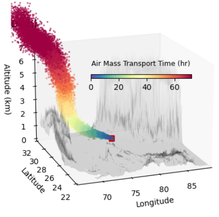
2. Load and Plot FLEXPART Trajectories

In trajectory mode, the output txt format information can be seen here
https://confluence.ecmwf.int/display/METV/FLEXPART+output

Column Number	Name	Unit	Description
1	time	s	The elapsed time in seconds since the middle point of the release interval
2	meanLon	degrees	Mean longitude position for all the particles
3	meanLat	degrees	Mean latitude position for all the particles
4	meanZ	m	Mean height for all the particles (above sea level)
5	meanTopo	m	Mean topography underlying all the particles
6	meanPBL	m	Mean PBL (Planetary Boundary Layer) height for all the particles (above ground level)
7	meanTropo	m	Mean tropopause height at the positions of particles (above sea level)
8	meanPv	PVU	Mean potential vorticity for all the particles
9	rmsHBefore	km	Total horizontal RMS (root mean square) distance before clustering
10	rmsHAfter	km	Total horizontal RMS distance after clustering
11	rmsVBefore	m	Total vertical RMS distance before clustering
12	rmsVAfter	m	Total vertical RMS distance after clustering
13	pblFract	%	Fraction of particles in the PBL
14	pv2Fract	%	Fraction of particles with PV < 2 PVU
15	tropoFract	%	Fraction of particles within the troposphere
16*	clLon_N	degrees	Mean longitude position for all the particles in cluster N
17*	clLat_N	degrees	Mean latitude position for all the particles in cluster N
18*	clZ_N	m	Mean height for all the particles in cluster N (above sea level)
19*	clFract_N	%	Fraction of particles in cluster N (above sea level)
20*	clRms_N	km	Total horizontal RMS distance in cluster N

input_file = "./data/retroplume_raw/traj/clustered_ind/2018-03-30-example.txt"
with open(input_file, "r") as file:
    lines = file.readlines()[7:]
data = [list(map(float, line.split())) for line in lines]
df_traj = pd.DataFrame(data, columns=columns[:len(data[0])])  # Adjust column count based on the actual data length

# 36 hr in total
kp_traj = df_traj[df_traj['receptor'] == 1.0].reset_index(drop = True)
dl_traj = df_traj[df_traj['receptor'] == 2.0].reset_index(drop = True)


trajectories = {
    "KP": {
        "lon": kp_traj['meanLon'],
        "lat": kp_traj['meanLat'],
        "alt": kp_traj['meanZ']/1000.0 + kp_traj['meanTopo']/1000.0,
        "time_delta": -1*(kp_traj['time'] - kp_traj['time'].iloc[0])/60/60.0,
    },
    "DL": {
        "lon": dl_traj['meanLon'],
        "lat": dl_traj['meanLat'],
        "alt": dl_traj['meanZ']/1000.0 + dl_traj['meanTopo']/1000.0,
        'time_delta':-1*(kp_traj['time'] - kp_traj['time'].iloc[0])/60/60.0
    },
}


elevation_interpolator = RegularGridInterpolator(
    (lat, lon), elevation / 1000.0  # Convert elevation to km
)

def set_3d_background(ax,sel_df_bio):
    ax.scatter(
    80.331871, 26.449923, 0.35,  # Kanpur at ground level
    zdir="z",
    marker="s",
    facecolor='none',
    edgecolor="b",
    s=40,
    alpha=1,lw = 2,
    label="Kanpur",zorder = 3
    )
    ax.scatter(
        77.069710, 28.679079, 0.53,  # New Delhi at ground level
        zdir="z",
        marker="s",
        facecolor='none',
        edgecolor="r",
        s=40,
        alpha=1,lw = 2,
        label="New Delhi",zorder = 3
    )

    # Plot the real-world elevation data as the base map
    ax.plot_surface(
        lon_grid,
        lat_grid,
        subset_elevation/1000.0,
        cmap=plt.cm.gray,#terrain_truncated,
        rstride=10,
        cstride=10,
        edgecolor='none',
        alpha=0.15,
    )
    
    
    
    # Customize grid appearance
    ax.xaxis._axinfo["grid"]["color"] = (1, 1, 1, 0)  # Transparent X grid
    ax.yaxis._axinfo["grid"]["color"] = (1, 1, 1, 0)  # Transparent Y grid
    ax.zaxis._axinfo["grid"]["color"] = (1, 1, 1, 0)  # Transparent Z grid
    ax.set_xlim([lon_min,lon_max])
    ax.set_ylim([lat_min, lat_max])
    ax.set_xlabel("Longitude")
    ax.set_ylabel("Latitude")
    ax.set_zlabel("Altitude (km)")



def plot_individual_day_traj(ax,traj):
#     colors = ['#97ff80','#679b4e','#ffe64c','#cd4040','purple','k']
#     time_categories = [0, 12,24, 48, 72, 96, 120]  # 5 days (0-24, 24-48, etc.)
#     for i in range(len(time_categories) - 1):
#         mask = (traj["time_delta"] >= time_categories[i]) & (traj["time_delta"] < time_categories[i + 1])
#         ax.plot(
#             np.array(traj["lon"])[mask],
#             np.array(traj["lat"])[mask],
#             np.array(traj["alt"])[mask],
#             color=colors[i],

#             linewidth=3.5,
#             label=f"<{time_categories[i+1]} hr",
#         )
    norm = mcolors.Normalize(vmin=0, vmax=72)  # Assuming time_delta ranges from 0 to 48 hours
    cmap = cm.get_cmap('Spectral_r')  # Choose a continuous colormap

    # Plot trajectories with continuous color representation

    for i in range(len(traj["time_delta"]) - 1):
        ax.plot(
            traj["lon"][i:i+2],
            traj["lat"][i:i+2],
            traj["alt"][i:i+2],
            color=cmap(norm(traj["time_delta"][i])),  # Map time_delta to color
            linewidth=2.5,zorder =15,
        )

# Create a 3D plot
fig = plt.figure(figsize=(6, 5))

norm = mcolors.Normalize(vmin=0, vmax=72)  # Assuming time_delta ranges from 0 to 48 hours
cmap = cm.get_cmap('Spectral_r')  # Choose a continuous colormap

ax = fig.add_subplot(111, projection='3d')
plot_individual_day_traj(ax, trajectories['DL'])
set_3d_background_dl(ax,sel_df_bio)
ax.set_zlim([0, 7])
ax.set_title('Delhi', loc = 'left', fontweight = 'bold',y=0.85)
ax.legend(ncol = 3, loc = (0.55, 0.45), fontsize = 8, frameon=True)
ax.view_init(elev=21, azim=-110)  # 

plt.show()

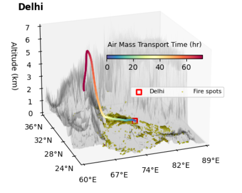
3.Particle Dispersion Illustration

import numpy as np

def plot_individual_day_traj_particles(ax, traj, n_particles=10, spread=0.05,initial_spread=0.05, final_spread=1):
    """
    Plot trajectory as particles instead of lines by generating points around the trajectory.
    
    Parameters:
    - ax: Matplotlib 3D axis.
    - traj: Dictionary with trajectory data (lon, lat, alt, time_delta).
    - n_particles: Number of particles to simulate per trajectory step.
    - spread: Standard deviation for particle dispersion around each step.
    """
    norm = mcolors.Normalize(vmin=0, vmax=72)  # Normalize time_delta
    cmap = cm.get_cmap('Spectral_r')  # Colormap for time
    
    # Loop through each trajectory point
    for i in range(len(traj["time_delta"])):
        
        current_spread = np.interp(
            traj["time_delta"][i], [0, max(traj["time_delta"])], [initial_spread, final_spread]
        )
        
        # Generate random offsets for particles
        lon_offsets = np.random.normal(traj["lon"][i], current_spread, n_particles)
        lat_offsets = np.random.normal(traj["lat"][i], current_spread, n_particles)
        alt_offsets = np.random.normal(traj["alt"][i], current_spread / 2, n_particles)  # Less spread for altitude
        
        # Get color for the current time_delta
        color = cmap(norm(traj["time_delta"][i]))
        
        # Plot the particles
        ax.scatter(
            lon_offsets,
            lat_offsets,
            alt_offsets,
            color=color,
            alpha=0.45,
            s=2,  # Small points for particles
        )


# Create a 3D plot
fig = plt.figure(figsize=(6, 5))

norm = mcolors.Normalize(vmin=0, vmax=72)  # Assuming time_delta ranges from 0 to 48 hours
cmap = cm.get_cmap('Spectral_r')  # Choose a continuous colormap

ax = fig.add_subplot(111, projection='3d')
plot_individual_day_traj_particles(ax, trajectories["DL"], n_particles=200, spread=0.25)
set_3d_background_dl(ax,df_pun)
ax.set_zlim([0, 7])
ax.set_title('Delhi', loc = 'left', fontweight = 'bold',y=0.85)
# ax.legend(ncol = 3, loc = (0.3, 0.7), fontsize = 8, frameon=True)
ax.view_init(elev=17, azim=-110)  # 

sm = cm.ScalarMappable(cmap=cmap, norm=norm)
axcolor = fig.add_axes([0.275, 0.6, 0.15, 0.015])  # Custom position and size for the colorbar axis
cbar = plt.colorbar(sm, cax=axcolor, orientation='horizontal')  # Create horizontal colorbar
cbar.set_label('Air Mass Transport Time (hr)', labelpad=-40, fontsize=9)     

plt.savefig("./Backward_trajectories_example_20181125_pollution_cases_particle_simulation_version.png", dpi =400)
plt.show()