OrbiTrack Dev Log 2: Dynamic M/Z Calibration

After reading m/z data from Orbitrap raw files, it is essential to perform m/z calibration based on known reference masses of internal calibrants.

For long-term measurements, especially those spanning days or weeks, dynamic calibration is critical, since m/z drift can occur over time, and calibration parameters from Day 1 may not hold by Day 7. The function below allows automated chunk-wise recalibration across retention time.

---

Dynamic M/Z Calibration Function

The function below performs dynamic m/z calibration using known calibrant ions. It splits the full dataset by identifying where the calibrant signals are strongest (typically their peak retention times), and fits a linear correction model within each chunk.

## Module 2 MS calibration
def calculate_ppm(observed_mass, ideal_mass):
    ppm = ((observed_mass - ideal_mass) / ideal_mass) * 1e6
    return ppm   

def find_peak_near_mass_after_mzcal(merged_spectrum, target_mass, tolerance_ppm):
    # Calculate the tolerance in m/z
    tolerance = target_mass * tolerance_ppm / 1e6
    
    # Find peaks within the tolerance range
    peaks_within_tolerance = merged_spectrum[
        (merged_spectrum['corrected_m/z'] >= target_mass - tolerance) &
        (merged_spectrum['corrected_m/z'] <= target_mass + tolerance)
    ]
    
    return peaks_within_tolerance    

def find_peak_near_mass(merged_spectrum, target_mass, tolerance_ppm):
    # Calculate the tolerance in m/z
    tolerance = target_mass * tolerance_ppm / 1e6
    
    # Find peaks within the tolerance range
    peaks_within_tolerance = merged_spectrum[
        (merged_spectrum['m/z'] >= target_mass - tolerance) &
        (merged_spectrum['m/z'] <= target_mass + tolerance)
    ]
    
    return peaks_within_tolerance    

def find_calibrant_matches(merged_spectrum, ideal_calibrants_mass, tolerance_ppm):
    calibrant_matches = []

    for ideal_mass in ideal_calibrants_mass:
        tolerance = ideal_mass * tolerance_ppm / 1e6  # Tolerance based on ppm
        peaks_within_tolerance = merged_spectrum[
            (merged_spectrum['m/z'] >= ideal_mass - tolerance) &
            (merged_spectrum['m/z'] <= ideal_mass + tolerance)
        ]
        
        if not peaks_within_tolerance.empty:
            # Store the actual masses and their RTs
            for _, peak in peaks_within_tolerance.iterrows():
                calibrant_matches.append((ideal_mass, peak['m/z'], peak['rt']))

    return calibrant_matches    

def find_rt_for_maximum_mz(merged_spectrum, ideal_calibrants_mass, tolerance_ppm,overlapped_scan):
    
    calibrant_matches = find_calibrant_matches(merged_spectrum, ideal_calibrants_mass, tolerance_ppm)
    
    if not calibrant_matches:
        print('No calibrants found in the spectrum.')
        return []
    
    max_ideal_mass = max(ideal_calibrants_mass)
    max_calibrant_matches = [(ideal_mass, actual_mass, rt) for ideal_mass, actual_mass, rt in calibrant_matches if ideal_mass == max_ideal_mass]    
    max_calibrant_rts = sorted([match[2] for match in max_calibrant_matches]) 
    
    # For overlapped mz scan, choose the second scan's rts (be careful!)
    if overlapped_scan == 1:
        max_calibrant_rts = max_calibrant_rts[1::2]
    return sorted(max_calibrant_rts)  # Sort the RTs

def correct_mz_dynamically(merged_spectrum, ideal_calibrants_mass, tolerance_ppm, overlapped_scan):
    merged_spectrum   = merged_spectrum.reset_index(drop = True)
    max_calibrant_rts = find_rt_for_maximum_mz(merged_spectrum, ideal_calibrants_mass, tolerance_ppm, overlapped_scan)
    chunk_boundaries = list(sorted(([merged_spectrum['rt'].min()] + max_calibrant_rts + [merged_spectrum['rt'].max()])))
    model_params = []
    # processing for each chunk split by the rts of the maximum m/z
    for i in range(len(chunk_boundaries) - 1):
        rt_start = chunk_boundaries[i]
        rt_end = chunk_boundaries[i + 1]
        chunk = merged_spectrum[(merged_spectrum['rt'] >= rt_start) & (merged_spectrum['rt'] < rt_end)]

        actual_masses = {}
        for ideal_mass in ideal_calibrants_mass:
            tolerance = ideal_mass * tolerance_ppm / 1e6
            peaks_within_chunk = chunk[
                (chunk['m/z'] >= ideal_mass - tolerance) &
                (chunk['m/z'] <= ideal_mass + tolerance)
            ]
            if not peaks_within_chunk.empty:
                actual_masses[ideal_mass] = np.mean(peaks_within_chunk['m/z'])

        # Step 5: Apply calibration if at least one calibrant is found
        if actual_masses:
            ideal_actual_pairs = np.array([(actual_masses[m], m) for m in actual_masses])
            
            weights = np.abs(1 - (ideal_actual_pairs[:, 0] / ideal_actual_pairs[:, 1]))  # Weight by proximity to ideal mass
            model = LinearRegression()
            model.fit(ideal_actual_pairs[:, 0].reshape(-1, 1), ideal_actual_pairs[:, 1], sample_weight=weights)

            # Apply the calibration to the current chunk
            chunk_rows = (merged_spectrum['rt'] >= rt_start) & (merged_spectrum['rt'] < rt_end)
            merged_spectrum.loc[chunk_rows, 'corrected_m/z'] = model.predict(merged_spectrum.loc[chunk_rows, 'm/z'].values.reshape(-1, 1))
            
            slope = model.coef_[0]
            intercept = model.intercept_
            model_params.append({'rt_start': rt_start, 'rt_end': rt_end, 'slope': slope, 'intercept': intercept})
    return merged_spectrum, model_params

Execution and Output Parameters

To address potential m/z drift over long measurement periods, I developed a dynamic calibration procedure that allows for chunk-wise m/z correction using varying fitting parameters. This approach avoids the limitations of applying a single static equation to the entire dataset and ensures more accurate mass alignment throughout the run.

A. Chunking by Retention Time of Maximum Calibrant

The full time series is segmented into chunks based on the retention time (RT) of the maximum calibrant ion.
Each chunk corresponds to a distinct time window, accounting for potential overlap to preserve peak continuity.
Note: In our untargeted direct infusion study, the retention time refers to the time stamp of each specific MS1 scan.

B. Calibrant-Based Correction Per Chunk

For each time chunk:

• The actual m/z values of selected calibrant ions are extracted.
• A linear regression is performed between the measured m/z values and their corresponding ideal masses.

This model is then used to recalibrate all ions in that chunk, shifting their m/z values to more accurate positions. Before the calibration

merged_spectrum_mzcal, model_params = correct_mz_dynamically(
    merged_spectrum, 
    ideal_calibrants_mass,
    calibration_tolerance_ppm,  # Predefined tolerance based on the typical mass error between actual and ideal calibrant values, I typically set to 20 ppm
    overlapped_scan_option
)

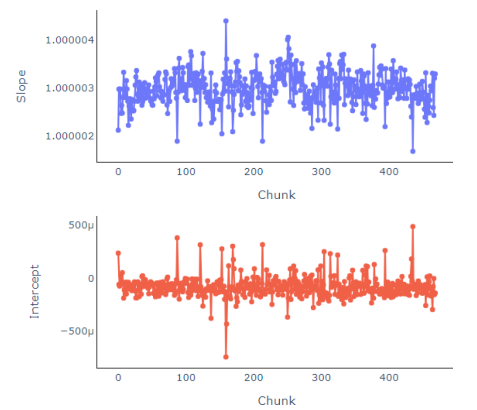
We then inspect the variation in calibration parameters (slope and intercept) across segments.

slope_ = []
intercept_ = []
for c in model_params:
    slope_.append(c['slope'])
    intercept_.append(c['intercept'])

fig = make_subplots(rows=1, cols=2)
fig.add_trace(go.Scatter(x=np.arange(len(slope_)), y=slope_, mode='lines+markers'), row=1, col=1)
fig.update_yaxes(title_text="Slope", col=1, row=1)
fig.add_trace(go.Scatter(x=np.arange(len(intercept_)), y=intercept_, mode='lines+markers'), row=1, col=2)
fig.update_yaxes(title_text="Intercept", col=2, row=1)
fig.update_xaxes(title_text="Chunk", showline=True, linecolor='black')
fig.update_layout(
    height=400, width=900,
    title_text="Dynamic Fitting Parameters Across Retention Time",
    plot_bgcolor='white', showlegend=False
)
fig.show()

Check Calibration Accuracy on Known Ions

We visualize the distribution of m/z values for five reference ions before and after correction. This comparison confirms the improvement in accuracy.

subplot_titles = ['Na2I', 'Na3I2', 'Na4I3','Na2[15]NO3', 'Na3[34]SO4']
masses = [172.88347, 322.77771, 472.67196, 108.9638, 166.9163]
colors = ['#447f44', '#cd4040', '#636efa', '#ddc927', '#9271dd']

subplot_titles = []
for i in range(len(masses)):
    ppm_differences = calculate_ppm(np.array(peak_results[masses[i]]['corrected_m/z']), masses[i])
    mean_ppm = np.mean(ppm_differences)
    subplot_titles.append(f"{['Na2I', 'Na3I2', 'Na4I3', 'Na2[15]NO3', 'Na3[34]SO4'][i]}: {mean_ppm:.2f} ppm")

fig = make_subplots(rows=1, cols=5, subplot_titles=subplot_titles)
for i in range(len(masses)):
    fig.add_trace(
        go.Histogram(x=peak_results[masses[i]]['corrected_m/z'], marker=dict(color='blue')),
        row=1, col=i+1
    )
    fig.add_trace(
        go.Histogram(x=peak_results[masses[i]]['m/z'], marker=dict(color='red', opacity=0.75)),
        row=1, col=i+1
    )
    fig.add_vline(x=masses[i], line_width=2, line_dash="dash", line_color="grey", row=1, col=i+1)
    fig.update_xaxes(title_text="m/z", range=[masses[i]-0.0025, masses[i]+0.0025], col=i+1, row=1)
    fig.update_yaxes(title_text="Count", col=i+1, row=1)

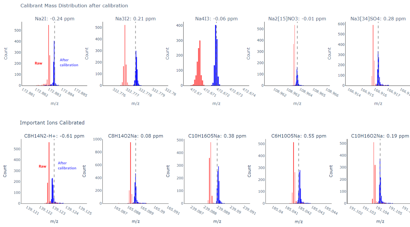
fig.update_layout(
    height=400, width=1500,
    title_text="Calibrant Mass Distribution Before and After Calibration",
    plot_bgcolor='white', showlegend=False
)
fig.show()

Here is an example of the post-check on those calibrants as well as those important ions (analytes).